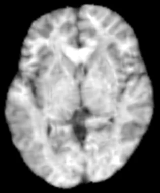
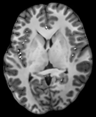
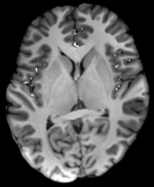
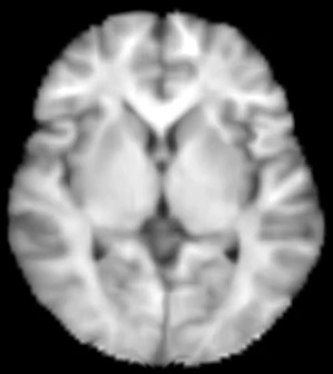
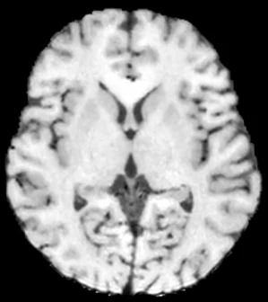
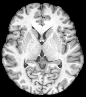
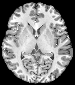
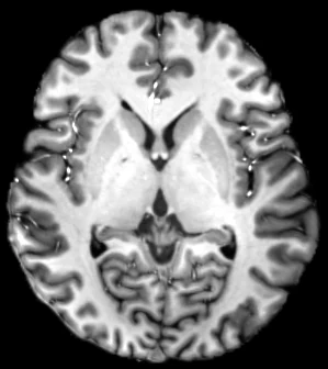
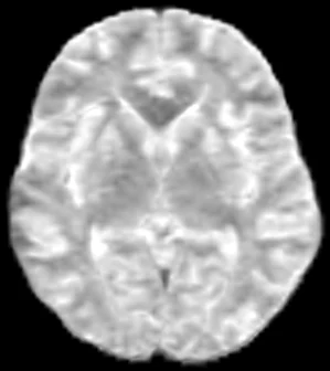
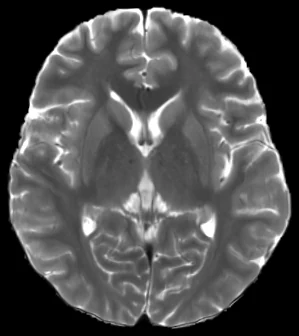
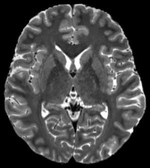
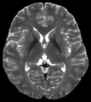
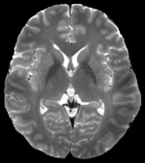
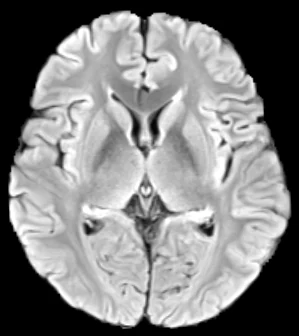
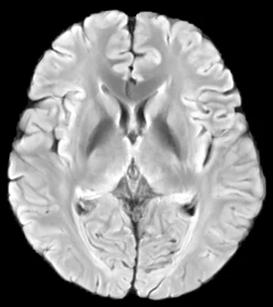
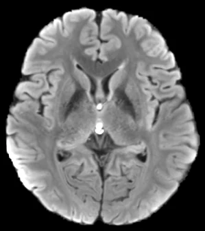
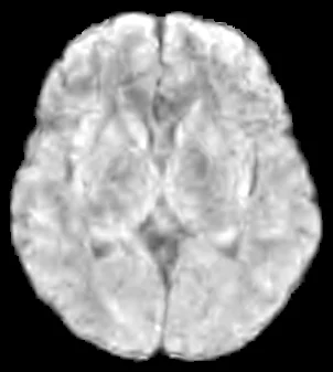
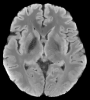
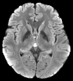
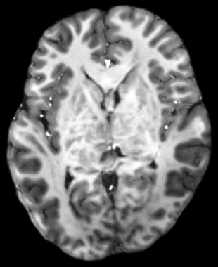
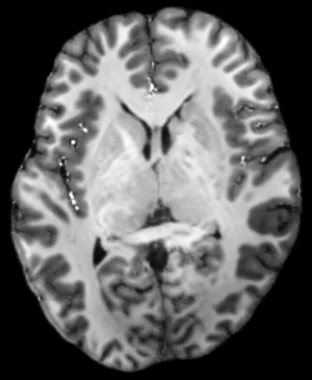
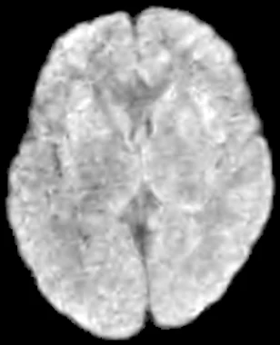
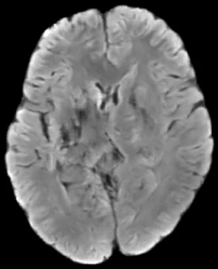
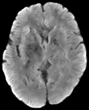
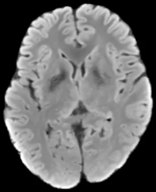
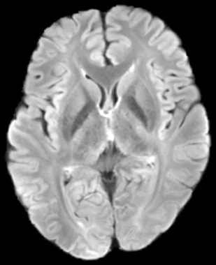
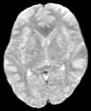
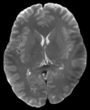
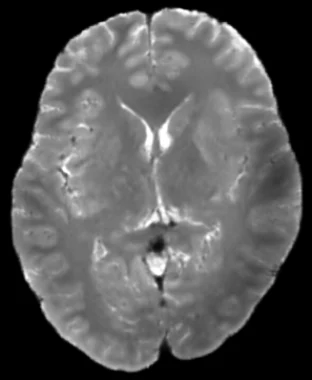
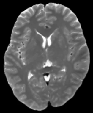
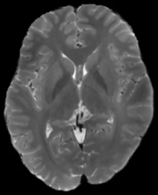
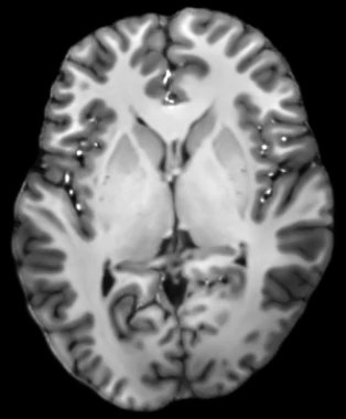
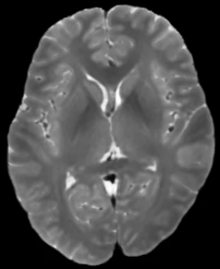
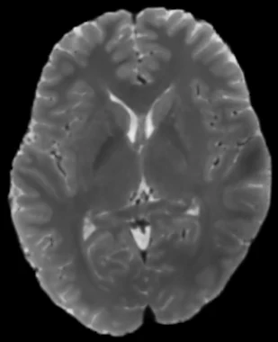
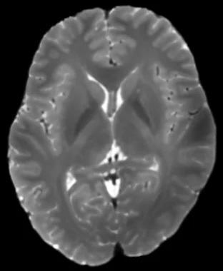
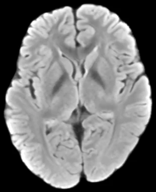
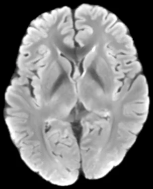
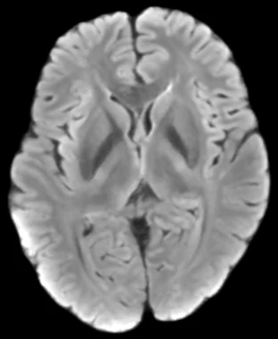
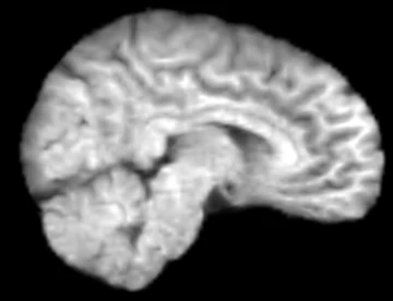
1st on Dice & VCboth anatomical metrics (0.907 / 0.917)
14 / 14deep-grey structures recovered from 0.1 T
TL;DR
FieldBridge turns a brain MRI acquired at
0.1, 1.5, 3 or 5 T into a 7 T-equivalent image.
Instead of one big generator jump, an unpaired Neural Schrödinger Bridge lets a
single time-conditioned network refine its own prediction over three steps. Trained almost
entirely on unpaired scans, fine-tuned on 660 paired slices, and calibrated with two post-hoc scalars per
contrast, it ranks 1st of 36 on the MRIxFields Task 1 validation
leaderboard — including first place on both anatomical metrics.
Drag to compare · example subject
Acquired 0.1 TFieldBridge → 7 T
Acquired 7 T · same subject
Background
The task: any field in, 7 T out
Magnetic field strength changes almost everything about an MR image at once — signal-to-noise,
achievable resolution, tissue contrast, B0/B1 homogeneity — and it changes
each contrast differently. Task 1 of the MRIxFields 2026 benchmark asks for a
single reference output: given a scan at 0.1, 1.5, 3 or 5 T, in any of three contrasts,
synthesise the 7 T-equivalent image while preserving the subject's anatomy.
One anatomy, five field strengths
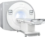
0.1 T
piMR-820H
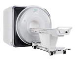
1.5 T
uMR 670
3 T
MAGNETOM Prisma
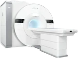
5 T
uMR Jupiter
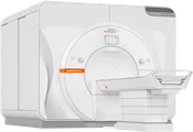
7 T
MAGNETOM Terra
T1w
T2w
T2 FLAIR
The same person scanned on five systems from three manufacturers,
registered to a common space.
Training data · unpaired
1,900+ cases
A different set of volunteers at every field.
0.1 T 1001.5 T 2283 T 1435 T 2667 T 319
Training data · paired
40 travelling volunteers
The same people scanned at all five fields × three contrasts — the benchmark's only true
pairs. Only 3 of them are in the training set: 660 paired slices to learn
from.
In training 3
Evaluation
5 metrics, 1 rank
Methods are ranked per metric; the five ranks are summed; lowest total
wins — consistency beats a single shiny number.
nRMSE ↓global intensity deviation
SSIM ↑structural preservation
LPIPS ↓perceptual realism
Dice ↑overlap, 14 deep-grey nuclei
Vol. cons. ↑regional volume agreement
Anatomical metrics use SynthSeg (Billot et al., Medical Image Analysis 2023) labels of 14
deep grey-matter structures. Challenge rules allow up to 12 separate models — one per input field ×
contrast — a freedom this method uses.
Method
An unpaired bridge, then twelve field-specific translators
FieldBridge keeps the content-preservation machinery of
CUT — PatchNCE and an
identity term — but replaces the single generator jump with a
Neural Schrödinger
Bridge: entropy-regularised optimal transport between the low-field and 7 T
distributions, unrolled as a short Markov chain. Training happens in two stages, followed by a
per-contrast calibration at inference.
Each step refines the predicted 7 T, not the source
The rollout: three refinements, one network
Follow it in order: from the low-field input, the same network
q_\phi(\cdot,\, t) predicts the 7 T image (top row), then the
next state blends that prediction back into the current one with a little noise (bottom row).
Three times, and the last prediction is the output.
During training, one t_i is drawn per iteration; earlier
iterates run under no_grad, so exactly one application of
q_\phi is back-propagated — a multi-step sampler for the price
of a one-step one.
1
Learning the field map without paired data
The whole unpaired cohort trains the step-conditioned translator — anatomy is held in place
patch by patch, not by a round trip.
PatchNCE anchors the anatomy patch by patch — green squares: same location,
same features — and the identity pass keeps real 7 T unchanged. All
\lambda at 1;
t_i \sim \mathcal{U}\{t_0, t_1, t_2\};
E and the projection head are discarded after this stage.
2
Fine-tuning on the 660 paired slices
Same rollout, but the final prediction is now compared directly with the acquired
7 T of the same subject.
x_0 low field
3-step rollout
\hat{x} synthesized 7 T
x_1 acquired 7 T, same subject
\mathcal{L}_{\mathrm{ft}} = \mathcal{L}_1 + 0.1\,\mathcal{L}_{\mathrm{LPIPS}} + 0.2\,\mathcal{L}_{\mathrm{SSIM}}40 epochs per cell
The extra input context below also enters here — no unpaired pre-training is
repeated.
What each slice sees: its neighbours and the other contrasts
With so few paired subjects, the cheapest extra information is more of the
same subject: adjacent slices add through-plane structure, and the other two contrasts —
already co-registered by the organisers — add complementary tissue information for free.
The input stack — up to 5 channels
Through-plane (2.5D)
s−1
slice s
s+1
Cross-contrast
T2w
FLAIR
W \leftarrow \tfrac{1}{n}\,[\,W, \ldots, W\,]first-convolution inflation — the forward pass is unchanged at initialisation, so
pre-training is never repeated
Who gets which channels
Which of a contrast's models keep their complementary-contrast
inputs — they matter most when the source is information-poor.
Source
2.5Dall models
Cross-contrast inputs
T1wmodel
T2wmodel
FLAIRmodel
0.1 T
✓
✓
✓
✓
1.5 T
✓
✓
✓
✓
3 T
✓
✕
✕
✓
5 T
✓
✕
✕
✓
At 3–5 T the source already carries most of the information — only
the T2-FLAIR model keeps its cross-contrast inputs, at every field. The ablation below
shows what each channel buys.
Twelve translators, three trained from scratch
Rules allow one model per input-field × contrast cell. Training all twelve
independently would cost ≈27 GPU-days; instead, each contrast trains once on its widest gap —
0.1 T → 7 T — and the other three fields warm-start from it.
trained from scratch on the widest gap of its contrast
Training time · 201 GPU-hours in total(≈ 8.4 GPU-days; ≈ 27 GPU-days at full budget)
Stage 1 from scratch · 150 h3 cells × 50 h · ≈ 50 epochs at 1.07 h
Warm start · 45 h9 cells × 5 h · 5 epochs each
Stage 2 fine-tuning · 4 h12 cells × 20 min
A warm start transfers everything — generator, discriminator, critic and projection head. Weights are never transferred across contrasts — a T1w model would still have
to learn FLAIR's inversion-recovery behaviour from scratch. Hardware: one NVIDIA RTX PRO 6000
Blackwell.
Inference: a per-contrast calibration fixes a systematic drift
Calibration factor by source field
\mu_{7\mathrm{T}} \,/\, \operatorname{mean}(\text{prediction}) over the brain mask — ×1.00 means no
correction needed.
T1wT2wT2 FLAIR
The direction of the drift is consistent across fields — a systematic bias,
not noise. T1w and FLAIR come out too dark, T2w too bright; FLAIR drifts ≈30% at
3–5 T.
Trained on distributions, the bridge has nothing pinning the absolute intensity
level. One scalar per contrast — the median 7 T brain mean over the prediction's
— repairs it, once per volume:
−12.1%nRMSE
−6.7%LPIPS
+1.1%SSIM
±0%Dice & volume consistency — SynthSeg is
contrast-randomised, so anatomy is untouched
A second scalar corrects dispersion rather than level: once the means
match, the best global scale still exceeds one where the predicted contrast is
compressed. Fitted leave-one-subject-out: ×1.069 T2w,
×1.021 FLAIR, T1w unchanged — post-processing, no retraining.
Results
First of 36 on the validation leaderboard
Every entry below is scored on the challenge server. The composite rank sums
the five per-metric ranks — the two anatomical metrics are where FieldBridge separates from the
field.
1st / 36
FieldBridge13
Team A15
Team B18
Team C26
CUT baseline90
Σ of the five per-metric ranks — lower is better. The starting point (CUT)
sums to 90; the full method reaches 13.
Task 1 validation leaderboard, top 5 of 36 entries + the CUT baseline.
Per-metric rank in parentheses; best value per column in bold. ↓ lower is better, ↑ higher is
better.
#
Method
nRMSE ↓
LPIPS ↓
SSIM ↑
Dice ↑
Vol. cons. ↑
Σ ranks ↓
1
FieldBridge (ours)
0.2595 (4)
0.0676 (3)
0.9244 (4)
0.9071 (1)
0.9168 (1)
13
2
Team A
0.2643 (5)
0.0637 (2)
0.9259 (3)
0.9064 (2)
0.9097 (3)
15
3
Team B
0.2591 (2)
0.0587 (1)
0.9293 (1)
0.8884 (7)
0.8828 (7)
18
4
Team C
0.2775 (6)
0.0704 (4)
0.9188 (6)
0.8890 (6)
0.8972 (4)
26
5
Team D
0.2880 (10)
0.0721 (5)
0.9137 (7)
0.9002 (4)
0.8869 (6)
32
—
CUT baseline
0.3041 (30)
0.0750 (10)
0.9053 (19)
0.8543 (14)
0.8601 (17)
90
Per-contrast scores (rank of 36)
— T2w draws our best raw scores but our worst ranks (everyone scores high there); T2-FLAIR, the
hardest input, gives the worst raw scores and the best ranks.
Contrast
nRMSE ↓
LPIPS ↓
SSIM ↑
Dice ↑
Vol. cons. ↑
T1w
0.2635 (4)
0.0641 (2)
0.9220 (4)
0.9127 (2)
0.9324 (2)
T2w
0.2205 (6)
0.0628 (6)
0.9349 (5)
0.9125 (4)
0.9062 (6)
T2 FLAIR
0.2945 (3)
0.0759 (3)
0.9163 (3)
0.8961 (1)
0.9117 (1)
Qualitative comparison — 0.1 T → 7 T
Acquired 0.1 T · input
CycleGAN · 0.1→7 T
CUT · 0.1→7 T
FieldBridge · ours
Acquired 7 T · target
Where to look — thalamus and putamen. CycleGAN and CUT
render the deep grey matter mottled and over-textured; FieldBridge keeps it homogeneous,
as in the acquired 7 T. At the cortex all three look plausible — which is exactly
why image-quality metrics separate the methods less than anatomical ones.
Acquired 0.1 T · input
CycleGAN · 0.1→7 T
CUT · 0.1→7 T
FieldBridge · ours
Acquired 7 T · target
The lowest-SNR input of the three. Both baselines invent
dark patches around the basal ganglia and in the deep white matter that don't exist in the
reference. FieldBridge keeps a consistent grey–white contrast — though its deep grey
remains flatter than the true 7 T.
Acquired 0.1 T · input
CycleGAN · 0.1→7 T
CUT · 0.1→7 T
FieldBridge · ours
Acquired 7 T · target
Our weakest contrast. Ventricles, CSF and the cortical
ribbon are recovered; the iron-rich dark nuclei and the finest cortical detail of
7 T are not fully reproduced.
Same subject in all panels. Every source field is compared further down the page.
Why the anatomical metrics favour the bridge
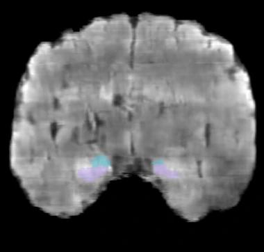
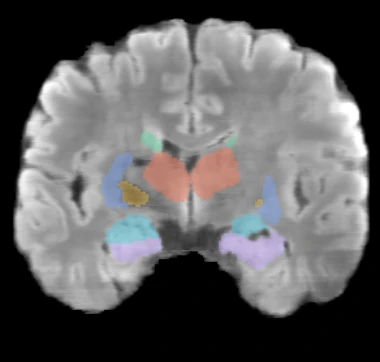
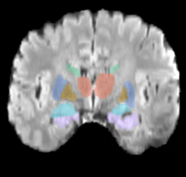
Run SynthSeg on the images and count what it finds. On this subject's
0.1 T acquisition, none of the 14 scored deep-grey structures are
detected. On the FieldBridge synthesis, all 14 are — with total volume within
0.5% of the acquired 7 T.
Acquired 0.1 T
0 / 14 · 0 vox
CycleGAN
3 / 14 · 280 vox
CUT
5 / 14 · 3,275 vox
FieldBridge · ours
14 / 14 · 55,306 vox
Acquired 7 T · reference
14 / 14 · 55,042 vox
Per-structure volume recovered
% of the 7 T volume that SynthSeg labels, axial T2w · same subject.
Acquired 0.1 TFieldBridge
Left thalamus40%86%
Caudate51%87%
Left pallidum23%74%
The pattern: structures without a CSF boundary — thalamus,
caudate, pallidum — are where 0.1 T loses the anatomy and where the translation
recovers most of it. The CSF-bounded hippocampus and amygdala keep a hard edge at any
field, so every method finds them.
The baselines mostly find only those two easy, CSF-bounded structures. FieldBridge restores
the boundaries SynthSeg needs everywhere else too — and it does so at the right size:
14 / 14structures recovered — on both subjects shown
+0.3% / +0.5%total deep-grey volume vs the acquired
7 T (the two subjects shown)
55.3k voxlabelled on our synthesis vs 55.0k on the
acquired 7 T — from 0 on the raw 0.1 T input
Explore the segmentation on the full volume, in 3-D, in the
interactive viewer.
Where each input channel helps
Relative improvement over a single-channel control
Same seed, schedule, inference and calibration — only the input stack differs.
A clean division of labour: through-plane
context drives the voxel and perceptual gains (nRMSE +7.4%, LPIPS +9.1%, Dice
untouched); complementary contrasts drive the anatomical
ones (Dice +3.1%, volume consistency +3.0%). T2-FLAIR is the exception — cross-contrast helps
it at every field. Absolute scores: nRMSE 0.289→0.265, LPIPS 0.075→0.065, Dice 0.867→0.894, VC
0.846→0.898.
How much does a better scanner buy?
from 0.1 T
from 1.5 T
from 3 T
from 5 T
acquired 7 T
T1w
T2w
T2 FLAIR
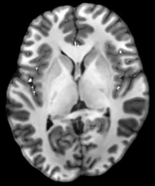
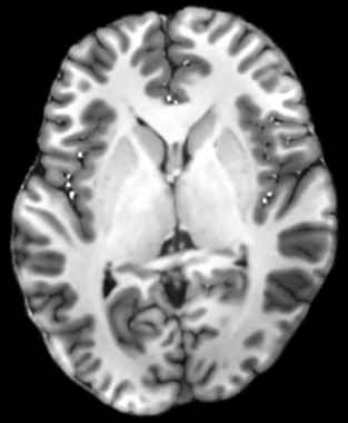
FieldBridge predictions of the same 7 T target from each source field,
next to the acquired 7 T. A stronger source helps — but far less than the field
ratio suggests: from a 0.1 T to a 5 T source, the perceptual distance (LPIPS) to
the target drops only ≈¼ on T1w and ≈½ on T2w. The value of source-field
information depends on the contrast.
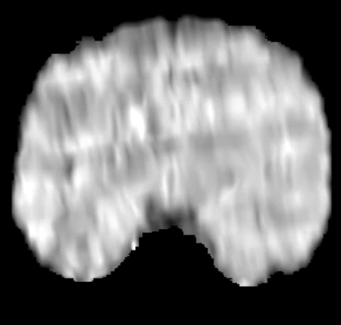
Slice-to-slice consistency
Inference runs on axial slices, so any slice-to-slice inconsistency shows up
as horizontal banding in a sagittal reformat. Δ is the mean absolute step in slice-mean intensity
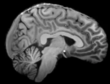
between consecutive slices — the acquired 7 T itself sits at 1.1%.
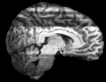
Acquired 0.1 Tinput
CycleGANΔ 2.3%
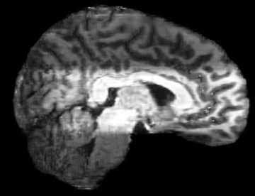
CUTΔ 3.9%
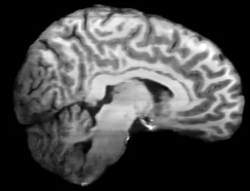
FieldBridgeΔ 1.8%
Acquired 7 TΔ 1.1% · floor
CUT shows heavy banding across the vertex and a step at the mid-brain; CycleGAN a
block break below the corpus callosum. Sharing one latent across the slices of a volume brings
FieldBridge to 1.8% — close to, but not yet at, the acquisition floor.
Conclusion
What we built for the challenge
FieldBridge turns a brain MRI acquired at 0.1, 1.5, 3 or 5 T into its
7 T-equivalent without any paired training data: an
Unpaired Neural
Schrödinger Bridge refines the prediction in three steps of one
time-conditioned network, learned on the unpaired cohort and fine-tuned on the
660 paired slices. It ranks 1st of 36 on the Task 1
validation leaderboard — first on both anatomical metrics — recovering all
14 scored deep-grey structures from a 0.1 T input within 0.5% of the
acquired 7 T by volume.